今回は基本的なことになりますが、フーリエ変換後の周波数領域のサイズを変更したら実画像のサイズがどうなるのか、次に中心周波数を少しずらしたどうなるのか、最後にMRIでよくあるパーシャルフーリエを試したことを記事にします。
周波数領域のサイズを変更してみた
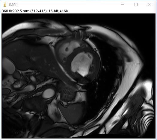
まず確認として、周波数領域のサイズを変更したらそれに応じて実画像のサイズも変わるのかを試してみました。今回も、前回と同じ以下の画像を用いて行います。
まずは、以下のコードで確認
import pydicom
import numpy as np
import matplotlib.pyplot as plt
img = pydicom.dcmread('IMG9')
pix_arr = img.pixel_array # 変数pix_arrにピクセルデータを格納
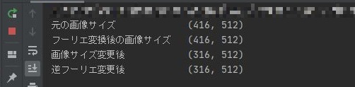
print('元の画像サイズ \t\t\t' + str(pix_arr.shape))
fft_arr = np.fft.fft2(pix_arr) # 変数fft_arrにpix_arrをフーリエ変換したデータを格納
fft_arr_shift = np.fft.fftshift(fft_arr)
print('フーリエ変換後の画像サイズ \t' + str(fft_arr_shift.shape))
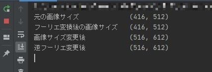
結果は

同一サイズになっています。それでは周波数領域の画像サイズを変更してみます。まずは、縮小です。
import pydicom
import numpy as np
import matplotlib.pyplot as plt

img = pydicom.dcmread('IMG9')
pix_arr = img.pixel_array # 変数pix_arrにピクセルデータを格納
print('元の画像サイズ \t\t\t' + str(pix_arr.shape))

fft_arr = np.fft.fft2(pix_arr) # 変数fft_arrにpix_arrをフーリエ変換したデータを格納
fft_arr_shift = np.fft.fftshift(fft_arr)
print('フーリエ変換後の画像サイズ \t' + str(fft_arr_shift.shape))

fft_arr_shift_size = fft_arr_shift[50 : fft_arr_shift.shape[0] - 50 , :]
print('画像サイズ変更後 \t\t\t' + str(fft_arr_shift_size.shape))

fft_rev = np.fft.fftshift(fft_arr_shift_size) # 位相シフトを戻す
fft_rev = np.fft.ifft2(fft_rev) #逆フーリエ変換
print('逆フーリエ変更後 \t\t\t' + str(fft_rev.shape))

fig = plt.figure()
ax1 = fig.add_subplot(1,4,1)
ax2 = fig.add_subplot(1,4,2)
ax3 = fig.add_subplot(1,4,3)
ax4 = fig.add_subplot(1,4,4)

ax1.imshow(pix_arr, cmap='gray')
ax2.imshow(np.abs(fft_arr_shift.real), cmap='gray', vmax =10000)
ax3.imshow(np.abs(fft_arr_shift_size.real), cmap='gray', vmax =10000)
ax4.imshow(np.abs(fft_rev.real), cmap='gray')

plt.show()
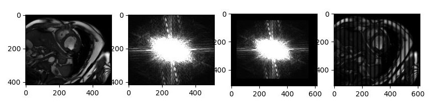
結果は
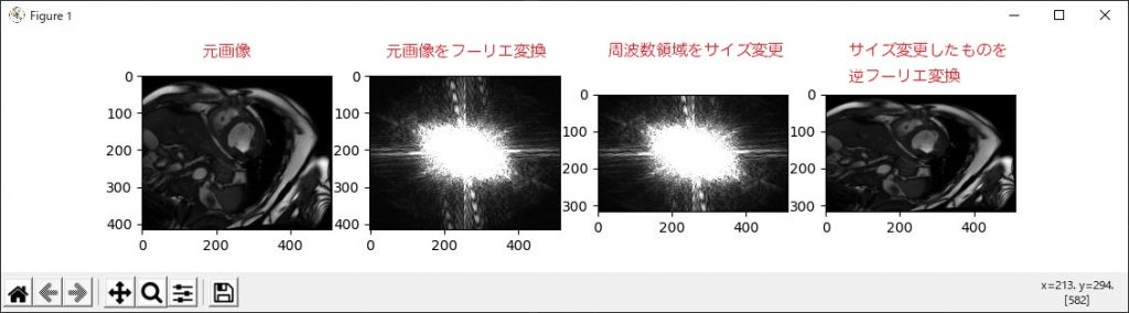
結果は、周波数領域をサイズを変えれば逆フーリエ変換した画像もサイズがかわる。あたりまえか・・・・
でも、面白いのが周波数領域のサイズを変更しても、実画像が切れるわけではなく、縮小されているのが面白いですね。。。。。(これも当たり前ですね。。)
今回は、縦方向の周波数領域を縮小しましたが、横方向に縮小しても同様の結果が起こります。
それでは、周波数領域のサイズを拡張したらどうなるのかなと思い試してみました。
元の画像サイズを100ピクセルずつ拡張して、その中心に元の周波数データを格納します。そしてそれを逆フーリエ変換しました。
import pydicom
import numpy as np
import matplotlib.pyplot as plt

img = pydicom.dcmread('IMG9')
pix_arr = img.pixel_array # 変数pix_arrにピクセルデータを格納
print('元の画像サイズ \t\t\t' + str(pix_arr.shape))

fft_arr = np.fft.fft2(pix_arr) # 変数fft_arrにpix_arrをフーリエ変換したデータを格納
fft_arr_shift = np.fft.fftshift(fft_arr)
print('フーリエ変換後の画像サイズ \t' + str(fft_arr_shift.shape))

fft_arr_shift_size = np.zeros((516,612),dtype = np.complex128)
fft_arr_shift_size[50:466, 50:562] = fft_arr_shift
print('画像サイズ変更後 \t\t\t' + str(fft_arr_shift_size.shape))

fft_rev = np.fft.fftshift(fft_arr_shift_size) # 位相シフトを戻す
fft_rev = np.fft.ifft2(fft_rev) #逆フーリエ変換
print('逆フーリエ変更後 \t\t\t' + str(fft_rev.shape))

fig = plt.figure()
ax1 = fig.add_subplot(1,4,1)
ax2 = fig.add_subplot(1,4,2)
ax3 = fig.add_subplot(1,4,3)
ax4 = fig.add_subplot(1,4,4)

ax1.imshow(pix_arr, cmap='gray')
ax2.imshow(np.abs(fft_arr_shift.real), cmap='gray', vmax =10000)
ax3.imshow(np.abs(fft_arr_shift_size.real), cmap='gray', vmax =10000)
ax4.imshow(np.abs(fft_rev.real), cmap='gray')

plt.show()
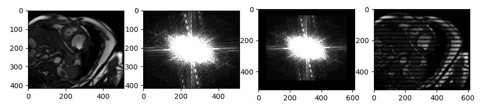
結果は
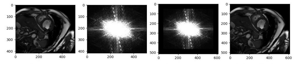
見えずらいかもしれませんが、周波数領域がきちんと拡張されており、それを逆フーリエ変換したものの画像サイズも大きくなっています。
結果、実画像と、フーリエ変換した画像サイズは同じ。周波数サイズを大きくして逆フーリエ変換すればその実画像のサイズも大きくなるという事でした。
位相を少しずらしてみた
今度は、位相を少しずらしてみたいと思います。
先ほどのコードで画像サイズを100ピクセル拡大した配列に元データを挿入したのですが、その位置を上下左右ずらしてみました。
まずは、横方向に10ピクセルずらしてみます。
上記コードの14行目を以下に変更します。
fft_arr_shift_size[50:466, 40:552] = fft_arr_shift
横方向にずらしたら縦方向に黒い線が現れました。
それでは、縦方向にずらしてみます。
fft_arr_shift_size[40:456, 50:562] = fft_arr_shift
今度は、横方向に黒い線が現れました。
今度はシフト量を変化してみます。
縞の間隔が狭くなりました。
原因は。。。。勉強不足でわかりません。誰か教えてください。でも、面白いですね。
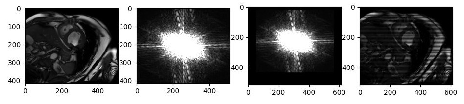
パーシャルフーリエを試してみた
最後に、MRIでよくあるパーシャルフーリエです。
撮像時間短縮のために、全データを収集するのではなく一部を収集して画像を作成するというものです。
周波数成分の下側20%程度の信号を0に書き換えてやってみます。
import pydicom
import numpy as np
import matplotlib.pyplot as plt

img = pydicom.dcmread('IMG9')
pix_arr = img.pixel_array # 変数pix_arrにピクセルデータを格納
print('元の画像サイズ \t\t\t' + str(pix_arr.shape))

fft_arr = np.fft.fft2(pix_arr) # 変数fft_arrにpix_arrをフーリエ変換したデータを格納
fft_arr_shift = np.fft.fftshift(fft_arr)
print('フーリエ変換後の画像サイズ \t' + str(fft_arr_shift.shape))

fft_arr_shift_par = np.ones(fft_arr_shift.shape,dtype=np.complex128)
fft_arr_shift_par = fft_arr_shift_par * fft_arr_shift #fft_arr_shiftをコピー
fft_arr_shift_par[320:,:] = 0
fft_rev = np.fft.fftshift(fft_arr_shift_par) # 位相シフトを戻す
fft_rev = np.fft.ifft2(fft_rev) #逆フーリエ変換

fig = plt.figure()
ax1 = fig.add_subplot(1,4,1)
ax2 = fig.add_subplot(1,4,2)
ax3 = fig.add_subplot(1,4,3)
ax4 = fig.add_subplot(1,4,4)

ax1.imshow(pix_arr, cmap='gray')
ax2.imshow(np.abs(fft_arr_shift.real), cmap='gray', vmax =10000)
ax3.imshow(np.abs(fft_arr_shift_par.real), cmap='gray', vmax =10000)
ax4.imshow(np.abs(fft_rev.real), cmap='gray')
plt.show()

おお!!きちんとできました。
正直、変な画像になるのかなと思っていたのですがきちんとできるものなのですね。
分解能とか確かめてみたいなと思うのですが、また今度の機会にしたいと思います。
最後に
今回は、周波数成分をいろいろといじってみた結果を記事にしてみました。
いいままで、周波数領域でいろいろとやるのは敷居が高く避けていたのですが今回やってみて、ちょっと苦手意識がなくなった気がします。
もし、興味がある方はやってみてください。
それでは、おつかれさまでした。